Tutorial

Mastering Python NumPy Indexing & Slicing: A Comprehensive Guide

Mastering Python NumPy Indexing & Slicing: A Comprehensive Guide

Today, we’re diving into a fundamental aspect of using NumPy effectively: indexing and slicing. Whether you’re analyzing data or processing images, understanding how to manipulate arrays efficiently is key. NumPy offers powerful tools to help you do just that. In this guide, we’ll explore the theory behind indexing and slicing, and then we’ll roll up our sleeves for some hands-on examples. Let’s jump right in! Understanding Indexing and Slicing Before we get into the details, let’s clarify what we mean by indexing and slicing: Understanding these concepts is crucial for working efficiently with arrays, enabling you to manipulate data quickly and effectively. Why Indexing and Slicing Matter Indexing and slicing in NumPy are much more flexible and powerful compared to Python lists. They allow for complex data extraction with minimal code and provide more control over your datasets. This is particularly useful in data analysis, where you often need to work with specific parts of your data. The Basics of Indexing Let’s start with the basics of indexing. Here’s how you can access elements in a NumPy array: One-Dimensional Arrays For a 1D array, indexing is straightforward: Indexing starts at 0, so the first element is accessed with index 0. Multi-Dimensional Arrays For multi-dimensional arrays, indexing uses a tuple of indices: Here, matrix[0, 0] accesses the element in the first row and first column. Negative Indexing NumPy supports negative indexing, which counts from the end of the array: Negative indexing is a convenient way to access elements relative to the end of an array. Advanced Indexing Techniques NumPy also provides advanced indexing capabilities, allowing for more complex data extraction: Boolean Indexing You can use boolean arrays to filter elements: Here, arr > 25 creates a boolean array indicating where the condition is true, and arr[bool_idx] extracts elements where the condition holds. Fancy Indexing Fancy indexing involves using arrays of indices to access elements: This allows you to select multiple elements from an array at once. The Art of Slicing Slicing enables you to extract portions of an array efficiently. The syntax for slicing is start:stop:step. One-Dimensional Slicing Let’s see slicing in action with a 1D array: Here, 1:4 specifies the start and stop indices (exclusive), extracting elements from index 1 to 3. Multi-Dimensional Slicing For multi-dimensional arrays, slicing can be applied along each dimension: This extracts the first two rows and the second and third columns. Step in Slicing You can also specify a step value to skip elements: Here, 0:5:2 extracts elements from index 0 to 4, taking every second element. Omitting Indices Omitting indices allows you to slice to the beginning or end of the array: This is a convenient shorthand for common slicing operations. Practical Applications of Indexing and Slicing Let’s apply what we’ve learned to a practical scenario. Consider a dataset representing temperatures over a week in different cities: In this example, we’ve efficiently accessed and filtered temperature data using indexing and slicing, highlighting how powerful these tools can be in data manipulation. Conclusion Mastering NumPy indexing and slicing is essential for anyone working with data in Python. By leveraging these techniques, you can extract, manipulate, and analyze your data with ease, unlocking the full potential of NumPy’s array capabilities. Next time you work with NumPy arrays, experiment with different indexing and slicing techniques to see how they can streamline your code and enhance your data analysis workflow. I hope this tutorial helps you gain a deeper understanding of NumPy indexing and slicing. Feel free to reach out with any questions or if you need further examples!

Mastering Python NumPy Indexing & Slicing: A Comprehensive Guide Read More »

Exploring Python NumPy Data Types: A Deep Dive

Exploring Python NumPy Data Types: A Deep Dive

Hey there, tech enthusiasts! If you’re delving into the world of Python for data science or any numerical computation, you’ve probably heard about NumPy. It’s that powerhouse library that makes Python incredibly efficient for numerical operations, especially when dealing with arrays and matrices. Today, we’re going to chat about NumPy data types, often called dtypes. Understanding these is crucial for optimizing performance and ensuring precision in your computations. Let’s get started! Why NumPy and Its Data Types Matter Before we dive into the specifics of data types, let’s quickly discuss why NumPy is so important. NumPy stands for “Numerical Python” and is the foundation for almost all advanced scientific computing in Python. It’s optimized for speed and has many powerful features that make handling numerical data a breeze. The secret sauce behind NumPy’s performance lies in its use of homogeneous data types. This means that all elements in a NumPy array must be of the same data type, allowing for efficient memory use and faster computations. A Tour of NumPy Data Types NumPy offers a wide array of data types, and each serves a specific purpose. Let’s take a look at some of the most commonly used ones: 1. Integer Types NumPy supports various integer types, differentiated by their bit size. The common ones include: These variations allow you to choose the most efficient size for your data, minimizing memory usage without sacrificing the range you need. 2. Unsigned Integer Types If you’re dealing with non-negative numbers, you might opt for unsigned integers: These are great when you need to maximize the positive range at the same bit size. 3. Floating Point Types Floating-point numbers are used for real numbers and come in a couple of flavors: Floating-point numbers can represent very large or very small numbers, making them ideal for scientific calculations. 4. Complex Number Types For complex numbers, NumPy provides: These are particularly useful in fields like electrical engineering and physics. 5. Boolean Type The boolean type (bool) represents True or False values, using only one bit per element. 6. String Types NumPy can handle string data, albeit with some limitations. You can specify a fixed size with S (e.g., S10 for strings up to 10 characters) or use U for Unicode strings (e.g., U10). Understanding How NumPy Uses Dtypes Now that we’ve gone through the types, let’s understand how NumPy uses them under the hood. When you create a NumPy array, you can specify the dtype explicitly: Specifying the dtype is essential for ensuring that your data is stored and computed efficiently. If you don’t specify a dtype, NumPy tries to infer it from the data you provide. Why Choosing the Right Dtype Matters Choosing the correct dtype can significantly impact both the memory consumption and the speed of your computations. Here’s why: Practical Example: Image Processing Let’s see how dtype selection affects a practical application like image processing. Images are typically stored as arrays of pixel values: Here, we use uint8 to represent pixel values because they naturally range from 0 to 255. Using a larger dtype would unnecessarily increase the memory footprint of our image data. Converting Between Dtypes NumPy makes it easy to convert between different data types using the astype method. This can be handy when preparing data for specific calculations: Be cautious with conversions, especially between integers and floats, as you may lose precision or encounter unexpected results due to rounding. Conclusion Understanding and effectively using NumPy data types is vital for any Python programmer working with numerical data. By choosing the appropriate dtype for your arrays, you can optimize your code for both speed and memory usage, ensuring your applications run efficiently. So, the next time you’re setting up your data structures with NumPy, remember to pay attention to those dtypes. They might seem like just a detail, but they can make a world of difference in your code’s performance. I hope this guide helps you get a solid grasp on NumPy data types and their significance in Python programming. If you have any questions or need further clarification, feel free to ask!

Exploring Python NumPy Data Types: A Deep Dive Read More »

Mastering Data Visualization with Matplotlib: An In-Depth Tutorial

Mastering Data Visualization with Matplotlib: An In-Depth Tutorial

Hey there, fellow data scientists! If you’re like me, you know that sometimes numbers alone just don’t cut it when you’re trying to explain your insights. That’s where data visualization steps in to save the day, and today, we’re going to take a deep dive into one of the most popular Python libraries for creating visualizations: Matplotlib. Whether you’re a seasoned data scientist or just dipping your toes into the world of data, Matplotlib is your trusty sidekick in making your data look pretty and, more importantly, understandable. By the end of this tutorial, you’ll be crafting beautiful plots and charts that not only impress but also inform. So, roll up your sleeves, open up your favorite Python editor, and let’s get plotting! Getting to Know Matplotlib First things first—what is Matplotlib? Simply put, Matplotlib is a powerful Python library used for creating static, animated, and interactive visualizations. It’s like the Swiss Army knife of plotting, allowing you to generate everything from simple line plots to complex interactive dashboards. Installing Matplotlib Before we can start creating amazing plots, we need to have Matplotlib installed. If you haven’t done this already, it’s as easy as pie. Just fire up your terminal or command prompt and run: Boom! You’re ready to go. Importing Matplotlib Now that we have Matplotlib installed, let’s bring it into our Python script. Typically, it’s imported using the alias plt, which keeps things concise and readable. Here’s how you do it: And with that, you’re all set up. Let’s dive into creating some plots! Basic Plotting with Matplotlib Let’s start with something simple: a line plot. Imagine you have some data that represents the temperature over a week, and you want to visualize this trend. Creating a Simple Line Plot Here’s how you can create a basic line plot in Matplotlib: This little script will pop up a window showing your line plot with days on the x-axis and temperatures on the y-axis. Easy, right? Customizing Plots Matplotlib gives you a ton of control over your plots. You can change colors, add labels, tweak line styles, and more. Let’s jazz up our line plot a bit: Here, we’ve changed the line color to purple, added circle markers at each data point, and set a dashed line style. We also increased the font size for the title and labels to make them stand out. Plotting Multiple Lines What if you have multiple datasets you want to compare on the same plot? Easy! Let’s say you also have data for the previous week: The label parameter is used here to distinguish between the two lines, and the plt.legend() function is called to display a legend on the plot. Advanced Plotting Techniques Okay, now that we have the basics down, let’s spice things up with some advanced plots. Matplotlib can handle scatter plots, bar plots, histograms, and more. Here’s how you can use them to get the most out of your data. Scatter Plots Scatter plots are great for showing relationships between two variables. For instance, if you’re analyzing the relationship between study hours and test scores, a scatter plot is your best friend. The scatter plot provides a clear visual of how test scores improve with more hours studied. Notice how easy it is to spot trends this way? Bar Plots Bar plots are perfect for comparing quantities across categories. Let’s say you want to visualize sales data for different products: The height of each bar corresponds to the sales numbers, giving a clear picture of which products are doing well. Histograms Histograms are useful for understanding the distribution of data points. For instance, if you’re analyzing the distribution of ages in a survey, a histogram can provide valuable insights. The bins parameter determines how the data is grouped, giving you control over the granularity of the distribution. Customization and Styling One of the best things about Matplotlib is how customizable it is. You can tweak almost every aspect of your plot to match your style or branding. Customizing Colors and Styles Want to match your plot to a specific color scheme? You can customize colors using color names, hex codes, or RGB values. Here’s an example: Using hex codes like #FF5733 allows for precise color matching. You can also adjust the grid lines for better readability. Adding Annotations Annotations can be used to highlight specific points or add notes to your plot, making your visualizations more informative. Annotations can guide the viewer’s attention to critical data points and provide context. Using Subplots Sometimes you want to display multiple plots side by side. Matplotlib’s subplots function makes it easy to create complex layouts. Subplots allow you to present related plots in a cohesive manner, making comparisons easy. Working with Figures and Axes Understanding the concepts of figures and axes is crucial when creating more sophisticated plots. Think of a figure as the overall window or canvas, while axes are the plots within that canvas. Understanding Figures and Axes In Matplotlib, the figure object holds everything together, and you can have multiple axes in a single figure. Here’s a simple example: Using plt.tight_layout() ensures that plots don’t overlap and everything looks neat. Adjusting Layouts Matplotlib offers several functions to fine-tune the layout of your plots. For example, plt.subplots_adjust() allows you to manually adjust the spacing between subplots. By adjusting the hspace and wspace parameters, you can customize the spacing between plots to your liking. Saving Figures Once you’ve created a beautiful plot, you might want to save it as an image file. Matplotlib makes this easy with the savefig() function. The dpi parameter sets the resolution of the saved image, and bbox_inches=’tight’ ensures there’s no extra whitespace. Creating Interactive and Animated Plots Matplotlib also supports interactive and animated plots, allowing for dynamic data exploration. Interactive Plots with mpl_toolkits For more interactive plots, you can use toolkits like mpl_toolkits.mplot3d for 3D plotting or other external libraries that integrate with Matplotlib, like mpl_interactions for interactive sliders and widgets. This example creates a

Mastering Data Visualization with Matplotlib: An In-Depth Tutorial Read More »

Scroll to Top
Contact Form Demo